Python实现随机森林RF模型超参数的优化详解

目录

• 1 代码分段讲解
• 1.1 数据与模型准备
• 1.2 超参数范围给定
• 1.3 超参数随机匹配择优
• 1.4 超参数遍历匹配择优
• 1.5 模型运行与精度评定
• 2 完整代码

本文介绍基于Python的随机森林（Random Forest，RF）回归代码，以及模型超参数（包括决策树个数与最大深度、最小分离样本数、最小叶子节点样本数、最大分离特征数等）自动优化的代码。

本文是在上一篇文章Python实现随机森林RF并对比自变量的重要性的基础上完成的，因此本次仅对随机森林模型超参数自动择优部分的代码加以详细解释；而数据准备、模型建立、精度评定等其他部分的代码详细解释，大家直接点击上述文章Python实现随机森林RF并对比自变量的重要性查看即可。

其中，关于基于MATLAB实现同样过程的代码与实战，大家可以点击查看文章MATLAB实现随机森林（RF）回归与自变量影响程度分析。

本文分为两部分，第一部分为代码的分段讲解，第二部分为完整代码。

1 代码分段讲解

1.1 数据与模型准备

本部分是对随机森林算法的数据与模型准备，由于在之前的博客中已经详细介绍过了，本文就不再赘述~大家直接查看文章Python实现随机森林RF并对比自变量的重要性即可。

import pydot
import numpy as np
import pandas as pd
import scipy.stats as stats
import matplotlib.pyplot as plt
from pprint import pprint
from sklearn import metrics
from openpyxl import load_workbook
from sklearn.tree import export_graphviz
from sklearn.ensemble import RandomForestRegressor
from sklearn.model_selection import GridSearchCV
from sklearn.model_selection import RandomizedSearchCV

# Attention! Data Partition
# Attention! One-Hot Encoding

train_data_path='G:/CropYield/03_DL/00_Data/AllDataAll_Train.csv'
test_data_path='G:/CropYield/03_DL/00_Data/AllDataAll_Test.csv'
write_excel_path='G:/CropYield/03_DL/05_NewML/ParameterResult_ML.xlsx'
tree_graph_dot_path='G:/CropYield/03_DL/05_NewML/tree.dot'
tree_graph_png_path='G:/CropYield/03_DL/05_NewML/tree.png'

random_seed=44
random_forest_seed=np.random.randint(low=1,high=230)

# Data import

train_data=pd.read_csv(train_data_path,header=0)
test_data=pd.read_csv(test_data_path,header=0)

# Separate independent and dependent variables

train_Y=np.array(train_data['Yield'])
train_X=train_data.drop(['ID','Yield'],axis=1)
train_X_column_name=list(train_X.columns)
train_X=np.array(train_X)

test_Y=np.array(test_data['Yield'])
test_X=test_data.drop(['ID','Yield'],axis=1)
test_X=np.array(test_X)

1.2 超参数范围给定

首先，我们需要对随机森林模型超参数各自的范围加以确定，之后我们将在这些范围内确定各个超参数的最终最优取值。换句话说，我们现在先给每一个需要择优的超参数划定一个很大很大的范围（例如对于“决策树个数”这个超参数，我们可以将其范围划定在10到5000这样一个很大的范围），然后后期将用择优算法在每一个超参数的这个范围内进行搜索。

在此，我们先要确定对哪些超参数进行择优。本文选择在随机森林算法中比较重要的几个超参数进行调优，分别是：决策树个数n_estimators，决策树最大深度max_depth，最小分离样本数（即拆分决策树节点所需的最小样本数）min_samples_split，最小叶子节点样本数（即一个叶节点所需包含的最小样本数）min_samples_leaf，最大分离特征数（即寻找最佳节点分割时要考虑的特征变量数量）max_features，以及是否进行随机抽样bootstrap等六种。关于上述超参数如果大家不是太了解具体的含义，可以查看文章Python实现随机森林RF并对比自变量的重要性的1.5部分，可能就会比较好理解了（不过其实不理解也不影响接下来的操作）。

这里提一句，其实随机森林的超参数并不止上述这些，我这里也是结合数据情况与最终的精度需求，选择了相对比较常用的几个超参数；大家依据各自实际需要，选择需要调整的超参数，并用同样的代码思路执行即可。

# Search optimal hyperparameter

n_estimators_range=[int(x) for x in np.linspace(start=50,stop=3000,num=60)]
max_features_range=['auto','sqrt']
max_depth_range=[int(x) for x in np.linspace(10,500,num=50)]
max_depth_range.append(None)
min_samples_split_range=[2,5,10]
min_samples_leaf_range=[1,2,4,8]
bootstrap_range=[True,False]

random_forest_hp_range={'n_estimators':n_estimators_range,
                        'max_features':max_features_range,
                        'max_depth':max_depth_range,
                        'min_samples_split':min_samples_split_range,
                        'min_samples_leaf':min_samples_leaf_range
                        # 'bootstrap':bootstrap_range
                        }
pprint(random_forest_hp_range)

可以看到，上述代码首先是对六种超参数划定了一个范围，然后将其分别存入了一个超参数范围字典random_forest_hp_range。在这里大家可以看到，我在存入字典时，将bootstrap的范围这一句注释掉了，这是由于当时运行后我发现bootstrap还是处于True这个状态比较好（也就是得到的结果精度比较高），因此就取消了这一超参数的择优；大家依据个人数据与模型的实际情况来即可~

我们可以看一下random_forest_hp_range变量的取值情况：

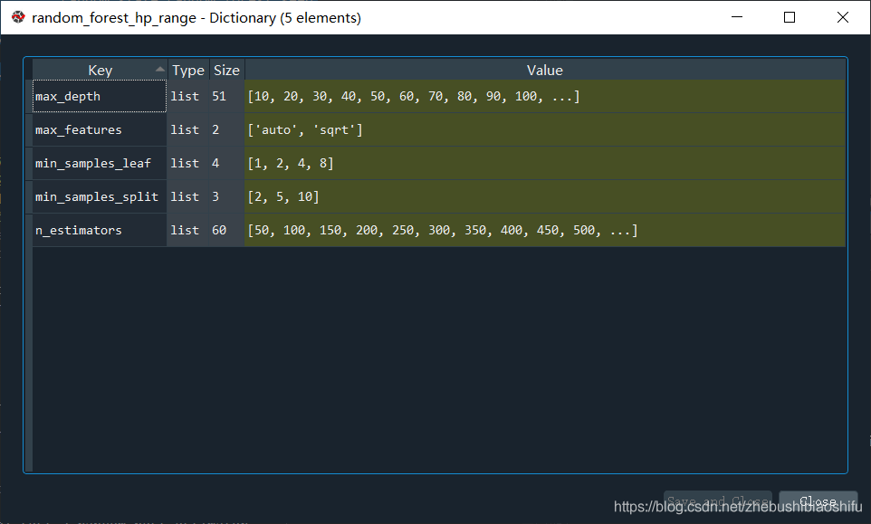
没错，它是一个字典，键就是超参数的名称，值就是超参数的范围。因为我将bootstrap注释掉了，因此这个字典里就没有bootstrap这一项了~

1.3 超参数随机匹配择优

上面我们确定了每一种超参数各自的范围，那么接下来我们就将他们分别组合，对比每一个超参数取值组合所得到的模型结果，从而确定最优超参数组合。

其实大家会发现，我们上面划定六种超参数（除去我后来删除的bootstrap的话是五种），如果按照排列组合来计算的话，会有很多很多种组合方式，如果要一一尝试未免也太麻烦了。因此，我们用到RandomizedSearchCV这一功能——其将随机匹配每一种超参数组合，并输出最优的组合。换句话说，我们用RandomizedSearchCV来进行随机的排列，而不是对所有的超参数排列组合方法进行遍历。这样子确实可以节省很多时间。

random_forest_model_test_base=RandomForestRegressor()
random_forest_model_test_random=RandomizedSearchCV(estimator=random_forest_model_test_base,
                                                   param_distributions=random_forest_hp_range,
                                                   n_iter=200,
                                                   n_jobs=-1,
                                                   cv=3,
                                                   verbose=1,
                                                   random_state=random_forest_seed
                                                   )
random_forest_model_test_random.fit(train_X,train_Y)

best_hp_now=random_forest_model_test_random.best_params_
pprint(best_hp_now)

由代码可以看到，我们首先建立一个随机森林模型random_forest_model_test_base，并将其带入到RandomizedSearchCV中；其中，RandomizedSearchCV的参数组合就是刚刚我们看的random_forest_hp_range，n_iter就是具体随机搭配超参数组合的次数（这个次数因此肯定是越大涵盖的组合数越多，效果越好，但是也越费时间），cv是交叉验证的折数（RandomizedSearchCV衡量每一种组合方式的效果就是用交叉验证来进行的），n_jobs与verbose是关于模型线程、日志相关的信息，大家不用太在意，random_state是随机森林中随机抽样的随机数种子。

之后，我们对random_forest_model_test_random加以训练，并获取其所得到的最优超参数匹配组合best_hp_now。在这里，模型的训练次数就是n_iter与cv的乘积（因为交叉验证有几折，那么就需要运行几次；而一共有n_iter个参数匹配组合，因此总次数就是二者相乘）。例如，用上述代码那么一共就需要运行600次。运行过程在程序中将自动显示，如下图。

可以看到，一共有600次fit，我这里共花了11.7min完成。具体速度和电脑配置、自变量与因变量数据量大小，以及电脑此时内存等等都有关。

运行完毕，我们来看看找到的最有超参数组合best_hp_now。

可以看到，经过200种组合匹配方式的计算，目前五种超参数最优的组合搭配方式已经得到了。其实每一次得到的超参数最优组合结果差距也是蛮大的——例如同一批数据，有的时候我得到的n_estimators最优值是如图所示的100，有的时候也会是2350；所以大家依据实际情况来判断即可~

那么接下来，我们就继续对这一best_hp_now所示的结果进行更进一步的择优。

1.4 超参数遍历匹配择优

刚刚我们基于RandomizedSearchCV，实现了200次的超参数随机匹配与择优；但是此时的结果是一个随机不完全遍历后所得的结果，因此其最优组合可能并不是全局最优的，而只是一个大概的最优范围。因此接下来，我们需要依据上述所得到的随机最优匹配结果，进行遍历全部组合的匹配择优。

遍历匹配即在随机匹配最优结果的基础上，在其临近范围内选取几个数值，并通过GridSearchCV对每一种匹配都遍历，从而选出比较好的超参数最终取值结果。

# Grid Search

random_forest_hp_range_2={'n_estimators':[60,100,200],
                          'max_features':[12,13],
                          'max_depth':[350,400,450],
                          'min_samples_split':[2,3] # Greater than 1
                          # 'min_samples_leaf':[1,2]
                          # 'bootstrap':bootstrap_range
                          }
random_forest_model_test_2_base=RandomForestRegressor()
random_forest_model_test_2_random=GridSearchCV(estimator=random_forest_model_test_2_base,
                                               param_grid=random_forest_hp_range_2,
                                               cv=3,
                                               verbose=1,
                                               n_jobs=-1)
random_forest_model_test_2_random.fit(train_X,train_Y)

best_hp_now_2=random_forest_model_test_2_random.best_params_
pprint(best_hp_now_2)

大家可以看到，本部分代码其实和1.3部分比较类似。我们着重讲解random_forest_hp_range_2。其中，n_estimators设定为了[60,100,200]，这是由于我们刚刚得到的best_hp_now中n_estimators为100，那么我们就在100附近选取几个值，作为新的n_estimators范围；max_features也是一样的，因为best_hp_now中max_features为'sqrt'，也就是输入数据特征（自变量）的个数的平方根，而我这里自变量个数大概是150多个，因此其开平方之后就是12.24左右，那么就选择其附近的两个数（需要为整数），因此就选择了[12,13]。其他的超参数取值也是类似的。这里我将'min_samples_leaf'也给注释掉了是因为我跑了很多次发现，'min_samples_leaf'还是取1最好，那么就直接选择为默认1（'min_samples_leaf'在不指定的情况下默认为1）即可，因为超参数范围越小，程序跑的就越快。

这里程序运行的次数就是每一种超参数取值个数的排列组合次数乘以交叉验证的折数，也就是(2*3*2*3)*3=108次，我们来看看是不是108次：

很明显，没有问题，就是108个fit。和前面的600次fit比起来，这样就快很多了（这也是为什么我直接将'min_samples_leaf'与'bootstrap'注释掉的原因；要是这两个超参数也参与的话，那么假设他们两个各有2个取值的话，总时间至少就要翻2*2=4倍）。

再来看看经过遍历择优后的最优超参数匹配取值best_hp_now_2。

以上就是我们经过一次随机择优、一次遍历择优之后的超参数结果（不要忘记了'min_samples_leaf'与'bootstrap'还要分别取1和True，也就是默认值）。如果大家感觉这个组合搭配还不是很好，那么可以继续执行本文“1.4 超参数遍历匹配择优”部分1到2次，精度可能会有更进一步的提升。

1.5 模型运行与精度评定

结束了上述超参数择优过程，我们就可以进行模型运行、精度评定与结果输出等操作。本部分内容除了第一句代码（将最优超参数组合分配给模型）之外，其余部分由于在之前的博客中已经详细介绍过了，本文就不再赘述~大家直接查看文章Python实现随机森林RF并对比自变量的重要性即可。

# Build RF regression model with optimal hyperparameters

random_forest_model_final=random_forest_model_test_2_random.best_estimator_

# Predict test set data

random_forest_predict=random_forest_model_test_2_random.predict(test_X)
random_forest_error=random_forest_predict-test_Y

# Draw test plot

plt.figure(1)
plt.clf()
ax=plt.axes(aspect='equal')
plt.scatter(test_Y,random_forest_predict)
plt.xlabel('True Values')
plt.ylabel('Predictions')
Lims=[0,10000]
plt.xlim(Lims)
plt.ylim(Lims)
plt.plot(Lims,Lims)
plt.grid(False)

plt.figure(2)
plt.clf()
plt.hist(random_forest_error,bins=30)
plt.xlabel('Prediction Error')
plt.ylabel('Count')
plt.grid(False)

# Verify the accuracy

random_forest_pearson_r=stats.pearsonr(test_Y,random_forest_predict)
random_forest_R2=metrics.r2_score(test_Y,random_forest_predict)
random_forest_RMSE=metrics.mean_squared_error(test_Y,random_forest_predict)**0.5
print('Pearson correlation coefficient is {0}, and RMSE is {1}.'.format(random_forest_pearson_r[0],
                                                                        random_forest_RMSE))

# Save key parameters

excel_file=load_workbook(write_excel_path)
excel_all_sheet=excel_file.sheetnames
excel_write_sheet=excel_file[excel_all_sheet[0]]
excel_write_sheet=excel_file.active
max_row=excel_write_sheet.max_row
excel_write_content=[random_forest_pearson_r[0],random_forest_R2,random_forest_RMSE,
                     random_seed,random_forest_seed]
for i in range(len(excel_write_content)):
        exec("excel_write_sheet.cell(max_row+1,i+1).value=excel_write_content[i]")
excel_file.save(write_excel_path)

# Draw decision tree visualizing plot

random_forest_tree=random_forest_model_final.estimators_[5]
export_graphviz(random_forest_tree,out_file=tree_graph_dot_path,
                feature_names=train_X_column_name,rounded=True,precision=1)
(random_forest_graph,)=pydot.graph_from_dot_file(tree_graph_dot_path)
random_forest_graph.write_png(tree_graph_png_path)

# Calculate the importance of variables

random_forest_importance=list(random_forest_model_final.feature_importances_)
random_forest_feature_importance=[(feature,round(importance,8))
                                  for feature, importance in zip(train_X_column_name,
                                                                 random_forest_importance)]
random_forest_feature_importance=sorted(random_forest_feature_importance,key=lambda x:x[1],reverse=True)
plt.figure(3)
plt.clf()
importance_plot_x_values=list(range(len(random_forest_importance)))
plt.bar(importance_plot_x_values,random_forest_importance,orientation='vertical')
plt.xticks(importance_plot_x_values,train_X_column_name,rotation='vertical')
plt.xlabel('Variable')
plt.ylabel('Importance')
plt.title('Variable Importances')

2 完整代码

本文所用完整代码如下。

# -*- coding: utf-8 -*-
"""
Created on Sun Mar 21 22:05:37 2021

@author: fkxxgis
"""

import pydot
import numpy as np
import pandas as pd
import scipy.stats as stats
import matplotlib.pyplot as plt
from pprint import pprint
from sklearn import metrics
from openpyxl import load_workbook
from sklearn.tree import export_graphviz
from sklearn.ensemble import RandomForestRegressor
from sklearn.model_selection import GridSearchCV
from sklearn.model_selection import RandomizedSearchCV

# Attention! Data Partition
# Attention! One-Hot Encoding

train_data_path='G:/CropYield/03_DL/00_Data/AllDataAll_Train.csv'
test_data_path='G:/CropYield/03_DL/00_Data/AllDataAll_Test.csv'
write_excel_path='G:/CropYield/03_DL/05_NewML/ParameterResult_ML.xlsx'
tree_graph_dot_path='G:/CropYield/03_DL/05_NewML/tree.dot'
tree_graph_png_path='G:/CropYield/03_DL/05_NewML/tree.png'

random_seed=44
random_forest_seed=np.random.randint(low=1,high=230)

# Data import

train_data=pd.read_csv(train_data_path,header=0)
test_data=pd.read_csv(test_data_path,header=0)

# Separate independent and dependent variables

train_Y=np.array(train_data['Yield'])
train_X=train_data.drop(['ID','Yield'],axis=1)
train_X_column_name=list(train_X.columns)
train_X=np.array(train_X)

test_Y=np.array(test_data['Yield'])
test_X=test_data.drop(['ID','Yield'],axis=1)
test_X=np.array(test_X)

# Search optimal hyperparameter

n_estimators_range=[int(x) for x in np.linspace(start=50,stop=3000,num=60)]
max_features_range=['auto','sqrt']
max_depth_range=[int(x) for x in np.linspace(10,500,num=50)]
max_depth_range.append(None)
min_samples_split_range=[2,5,10]
min_samples_leaf_range=[1,2,4,8]
bootstrap_range=[True,False]

random_forest_hp_range={'n_estimators':n_estimators_range,
                        'max_features':max_features_range,
                        'max_depth':max_depth_range,
                        'min_samples_split':min_samples_split_range,
                        'min_samples_leaf':min_samples_leaf_range
                        # 'bootstrap':bootstrap_range
                        }
pprint(random_forest_hp_range)

random_forest_model_test_base=RandomForestRegressor()
random_forest_model_test_random=RandomizedSearchCV(estimator=random_forest_model_test_base,
                                                   param_distributions=random_forest_hp_range,
                                                   n_iter=200,
                                                   n_jobs=-1,
                                                   cv=3,
                                                   verbose=1,
                                                   random_state=random_forest_seed
                                                   )
random_forest_model_test_random.fit(train_X,train_Y)

best_hp_now=random_forest_model_test_random.best_params_
pprint(best_hp_now)

# Grid Search

random_forest_hp_range_2={'n_estimators':[60,100,200],
                          'max_features':[12,13],
                          'max_depth':[350,400,450],
                          'min_samples_split':[2,3] # Greater than 1
                          # 'min_samples_leaf':[1,2]
                          # 'bootstrap':bootstrap_range
                          }
random_forest_model_test_2_base=RandomForestRegressor()
random_forest_model_test_2_random=GridSearchCV(estimator=random_forest_model_test_2_base,
                                               param_grid=random_forest_hp_range_2,
                                               cv=3,
                                               verbose=1,
                                               n_jobs=-1)
random_forest_model_test_2_random.fit(train_X,train_Y)

best_hp_now_2=random_forest_model_test_2_random.best_params_
pprint(best_hp_now_2)

# Build RF regression model with optimal hyperparameters

random_forest_model_final=random_forest_model_test_2_random.best_estimator_

# Predict test set data

random_forest_predict=random_forest_model_test_2_random.predict(test_X)
random_forest_error=random_forest_predict-test_Y

# Draw test plot

plt.figure(1)
plt.clf()
ax=plt.axes(aspect='equal')
plt.scatter(test_Y,random_forest_predict)
plt.xlabel('True Values')
plt.ylabel('Predictions')
Lims=[0,10000]
plt.xlim(Lims)
plt.ylim(Lims)
plt.plot(Lims,Lims)
plt.grid(False)

plt.figure(2)
plt.clf()
plt.hist(random_forest_error,bins=30)
plt.xlabel('Prediction Error')
plt.ylabel('Count')
plt.grid(False)

# Verify the accuracy

random_forest_pearson_r=stats.pearsonr(test_Y,random_forest_predict)
random_forest_R2=metrics.r2_score(test_Y,random_forest_predict)
random_forest_RMSE=metrics.mean_squared_error(test_Y,random_forest_predict)**0.5
print('Pearson correlation coefficient is {0}, and RMSE is {1}.'.format(random_forest_pearson_r[0],
                                                                        random_forest_RMSE))

# Save key parameters

excel_file=load_workbook(write_excel_path)
excel_all_sheet=excel_file.sheetnames
excel_write_sheet=excel_file[excel_all_sheet[0]]
excel_write_sheet=excel_file.active
max_row=excel_write_sheet.max_row
excel_write_content=[random_forest_pearson_r[0],random_forest_R2,random_forest_RMSE,
                     random_seed,random_forest_seed]
for i in range(len(excel_write_content)):
        exec("excel_write_sheet.cell(max_row+1,i+1).value=excel_write_content[i]")
excel_file.save(write_excel_path)

# Draw decision tree visualizing plot

random_forest_tree=random_forest_model_final.estimators_[5]
export_graphviz(random_forest_tree,out_file=tree_graph_dot_path,
                feature_names=train_X_column_name,rounded=True,precision=1)
(random_forest_graph,)=pydot.graph_from_dot_file(tree_graph_dot_path)
random_forest_graph.write_png(tree_graph_png_path)

# Calculate the importance of variables

random_forest_importance=list(random_forest_model_final.feature_importances_)
random_forest_feature_importance=[(feature,round(importance,8))
                                  for feature, importance in zip(train_X_column_name,
                                                                 random_forest_importance)]
random_forest_feature_importance=sorted(random_forest_feature_importance,key=lambda x:x[1],reverse=True)
plt.figure(3)
plt.clf()
importance_plot_x_values=list(range(len(random_forest_importance)))
plt.bar(importance_plot_x_values,random_forest_importance,orientation='vertical')
plt.xticks(importance_plot_x_values,train_X_column_name,rotation='vertical')
plt.xlabel('Variable')
plt.ylabel('Importance')
plt.title('Variable Importances')

以上就是Python实现随机森林RF模型超参数的优化详解的详细内容，更多关于Python随机森林模型超参数优化的资料请关注我们其它相关文章！