python SVM 线性分类模型的实现

运行环境：win10 64位 py 3.6 pycharm 2018.1.1

导入对应的包和数据

import matplotlib.pyplot as plt
import numpy as np
from sklearn import datasets,linear_model,cross_validation,svm
def load_data_regression():
  diabetes = datasets.load_diabetes()
  return cross_validation.train_test_split(diabetes,diabetes.target,test_size=0.25,random_state=0)
def load_data_classfication():
  iris = datasets.load_iris()
  X_train = iris.data
  y_train = iris.target
  return cross_validation.train_test_split(X_train,y_train,test_size=0.25,random_state=0,stratify=y_train)

#线性分类SVM
def test_LinearSVC(*data):
  X_train,X_test,y_train,y_test = data
  cls = svm.LinearSVC()
  cls.fit(X_train,y_train)
  print('Coefficients:%s,intercept%s'%(cls.coef_,cls.intercept_))
  print('Score:%.2f'%cls.score(X_test,y_test))
X_train,X_test,y_train,y_test = load_data_classfication()
test_LinearSVC(X_train,X_test,y_train,y_test)

def test_LinearSVC_loss(*data):
  X_train,X_test,y_train,y_test = data
  losses = ['hinge','squared_hinge']
  for loss in losses:
    cls = svm.LinearSVC(loss=loss)
    cls.fit(X_train,y_train)
    print('loss:%s'%loss)
    print('Coefficients:%s,intercept%s'%(cls.coef_,cls.intercept_))
    print('Score:%.2f'%cls.score(X_test,y_test))
X_train,X_test,y_train,y_test = load_data_classfication()
test_LinearSVC_loss(X_train,X_test,y_train,y_test)

#考察罚项形式的影响
def test_LinearSVC_L12(*data):
  X_train,X_test,y_train,y_test = data
  L12 = ['l1','l2']
  for p in L12:
    cls = svm.LinearSVC(penalty=p,dual=False)
    cls.fit(X_train,y_train)
    print('penalty:%s'%p)
    print('Coefficients:%s,intercept%s'%(cls.coef_,cls.intercept_))
    print('Score:%.2f'%cls.score(X_test,y_test))
X_train,X_test,y_train,y_test = load_data_classfication()
test_LinearSVC_L12(X_train,X_test,y_train,y_test)

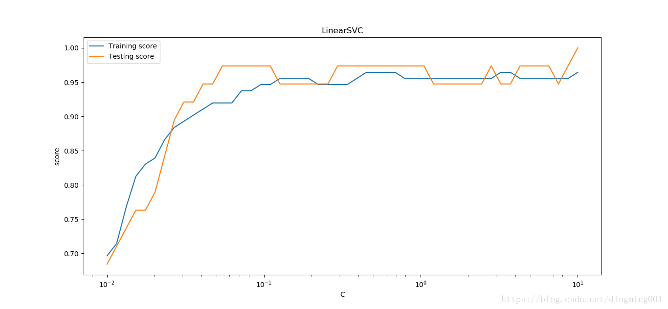
#考察罚项系数C的影响
def test_LinearSVC_C(*data):
  X_train,X_test,y_train,y_test = data
  Cs = np.logspace(-2,1)
  train_scores = []
  test_scores = []
  for C in Cs:
    cls = svm.LinearSVC(C=C)
    cls.fit(X_train,y_train)
    train_scores.append(cls.score(X_train,y_train))
    test_scores.append(cls.score(X_test,y_test))
  fig = plt.figure()
  ax = fig.add_subplot(1,1,1)
  ax.plot(Cs,train_scores,label = 'Training score')
  ax.plot(Cs,test_scores,label = 'Testing score')
  ax.set_xlabel(r'C')
  ax.set_xscale('log')
  ax.set_ylabel(r'score')
  ax.set_title('LinearSVC')
  ax.legend(loc='best')
  plt.show()
X_train,X_test,y_train,y_test = load_data_classfication()
test_LinearSVC_C(X_train,X_test,y_train,y_test)

#非线性分类SVM
#线性核
def test_SVC_linear(*data):
  X_train, X_test, y_train, y_test = data
  cls = svm.SVC(kernel='linear')
  cls.fit(X_train,y_train)
  print('Coefficients:%s,intercept%s'%(cls.coef_,cls.intercept_))
  print('Score:%.2f'%cls.score(X_test,y_test))
X_train,X_test,y_train,y_test = load_data_classfication()
test_SVC_linear(X_train,X_test,y_train,y_test)

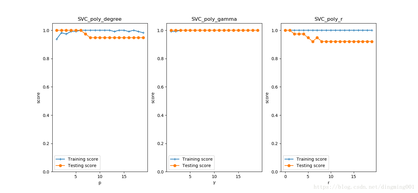
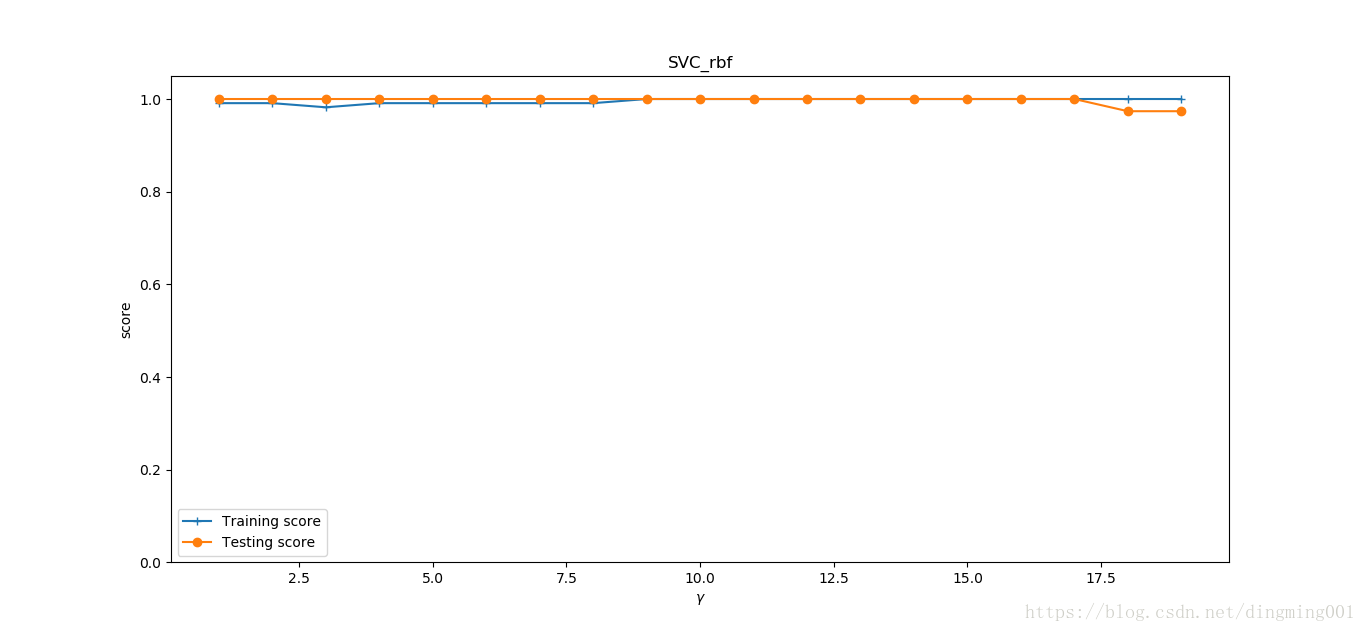
#考察高斯核
def test_SVC_rbf(*data):
  X_train, X_test, y_train, y_test = data
  ###测试gamm###
  gamms = range(1, 20)
  train_scores = []
  test_scores = []
  for gamm in gamms:
    cls = svm.SVC(kernel='rbf', gamma=gamm)
    cls.fit(X_train, y_train)
    train_scores.append(cls.score(X_train, y_train))
    test_scores.append(cls.score(X_test, y_test))
  fig = plt.figure()
  ax = fig.add_subplot(1, 1, 1)
  ax.plot(gamms, train_scores, label='Training score', marker='+')
  ax.plot(gamms, test_scores, label='Testing score', marker='o')
  ax.set_xlabel(r'$\gamma$')
  ax.set_ylabel(r'score')
  ax.set_ylim(0, 1.05)
  ax.set_title('SVC_rbf')
  ax.legend(loc='best')
  plt.show()
X_train,X_test,y_train,y_test = load_data_classfication()
test_SVC_rbf(X_train,X_test,y_train,y_test)

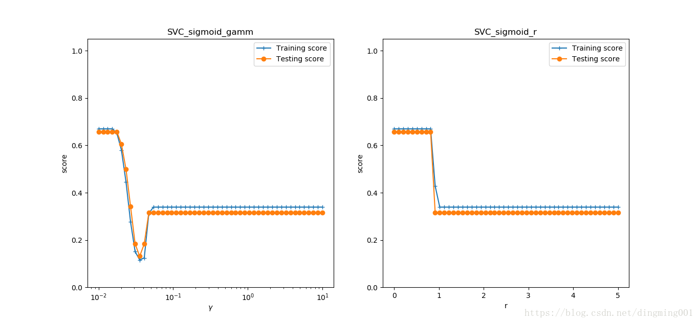
#考察sigmoid核
def test_SVC_sigmod(*data):
  X_train, X_test, y_train, y_test = data
  fig = plt.figure()
  ###测试gamm###
  gamms = np.logspace(-2, 1)
  train_scores = []
  test_scores = []
  for gamm in gamms:
    cls = svm.SVC(kernel='sigmoid',gamma=gamm,coef0=0)
    cls.fit(X_train, y_train)
    train_scores.append(cls.score(X_train, y_train))
    test_scores.append(cls.score(X_test, y_test))
  ax = fig.add_subplot(1, 2, 1)
  ax.plot(gamms, train_scores, label='Training score', marker='+')
  ax.plot(gamms, test_scores, label='Testing score', marker='o')
  ax.set_xlabel(r'$\gamma$')
  ax.set_ylabel(r'score')
  ax.set_xscale('log')
  ax.set_ylim(0, 1.05)
  ax.set_title('SVC_sigmoid_gamm')
  ax.legend(loc='best')

  #测试r
  rs = np.linspace(0,5)
  train_scores = []
  test_scores = []
  for r in rs:
    cls = svm.SVC(kernel='sigmoid', gamma=0.01, coef0=r)
    cls.fit(X_train, y_train)
    train_scores.append(cls.score(X_train, y_train))
    test_scores.append(cls.score(X_test, y_test))
  ax = fig.add_subplot(1, 2, 2)
  ax.plot(rs, train_scores, label='Training score', marker='+')
  ax.plot(rs, test_scores, label='Testing score', marker='o')
  ax.set_xlabel(r'r')
  ax.set_ylabel(r'score')
  ax.set_ylim(0, 1.05)
  ax.set_title('SVC_sigmoid_r')
  ax.legend(loc='best')
  plt.show()
X_train,X_test,y_train,y_test = load_data_classfication()
test_SVC_sigmod(X_train,X_test,y_train,y_test)

以上就是本文的全部内容，希望对大家的学习有所帮助，也希望大家多多支持我们。