keras CNN卷积核可视化,热度图教程

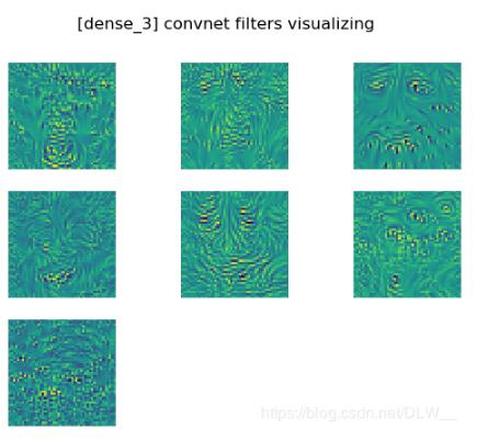
卷积核可视化

import matplotlib.pyplot as plt
import numpy as np
from keras import backend as K
from keras.models import load_model

# 将浮点图像转换成有效图像
def deprocess_image(x):
 # 对张量进行规范化
 x -= x.mean()
 x /= (x.std() + 1e-5)
 x *= 0.1
 x += 0.5
 x = np.clip(x, 0, 1)
 # 转化到RGB数组
 x *= 255
 x = np.clip(x, 0, 255).astype('uint8')
 return x

# 可视化滤波器
def kernelvisual(model, layer_target=1, num_iterate=100):
 # 图像尺寸和通道
 img_height, img_width, num_channels = K.int_shape(model.input)[1:4]
 num_out = K.int_shape(model.layers[layer_target].output)[-1]

 plt.suptitle('[%s] convnet filters visualizing' % model.layers[layer_target].name)

 print('第%d层有%d个通道' % (layer_target, num_out))
 for i_kernal in range(num_out):
  input_img = model.input
  # 构建一个损耗函数，使所考虑的层的第n个滤波器的激活最大化，-1层softmax层
  if layer_target == -1:
   loss = K.mean(model.output[:, i_kernal])
  else:
   loss = K.mean(model.layers[layer_target].output[:, :, :, i_kernal]) # m*28*28*128
  # 计算图像对损失函数的梯度
  grads = K.gradients(loss, input_img)[0]
  # 效用函数通过其L2范数标准化张量
  grads /= (K.sqrt(K.mean(K.square(grads))) + 1e-5)
  # 此函数返回给定输入图像的损耗和梯度
  iterate = K.function([input_img], [loss, grads])
  # 从带有一些随机噪声的灰色图像开始
  np.random.seed(0)
  # 随机图像
  # input_img_data = np.random.randint(0, 255, (1, img_height, img_width, num_channels)) # 随机
  # input_img_data = np.zeros((1, img_height, img_width, num_channels)) # 零值
  input_img_data = np.random.random((1, img_height, img_width, num_channels)) * 20 + 128. # 随机灰度
  input_img_data = np.array(input_img_data, dtype=float)
  failed = False
  # 运行梯度上升
  print('####################################', i_kernal + 1)
  loss_value_pre = 0
  # 运行梯度上升num_iterate步
  for i in range(num_iterate):
   loss_value, grads_value = iterate([input_img_data])
   if i % int(num_iterate/5) == 0:
    print('Iteration %d/%d, loss: %f' % (i, num_iterate, loss_value))
    print('Mean grad: %f' % np.mean(grads_value))
    if all(np.abs(grads_val) < 0.000001 for grads_val in grads_value.flatten()):
     failed = True
     print('Failed')
     break
    if loss_value_pre != 0 and loss_value_pre > loss_value:
     break
    if loss_value_pre == 0:
     loss_value_pre = loss_value
    # if loss_value > 0.99:
    #  break
   input_img_data += grads_value * 1 # e-3
  img_re = deprocess_image(input_img_data[0])
  if num_channels == 1:
   img_re = np.reshape(img_re, (img_height, img_width))
  else:
   img_re = np.reshape(img_re, (img_height, img_width, num_channels))
  plt.subplot(np.ceil(np.sqrt(num_out)), np.ceil(np.sqrt(num_out)), i_kernal + 1)
  plt.imshow(img_re) # , cmap='gray'
  plt.axis('off')

 plt.show()

运行

model = load_model('train3.h5')
kernelvisual(model,-1) # 对最终输出可视化
kernelvisual(model,6) # 对第二个卷积层可视化

热度图

import cv2
import matplotlib.pyplot as plt
import numpy as np
from keras import backend as K
from keras.preprocessing import image

def heatmap(model, data_img, layer_idx, img_show=None, pred_idx=None):
 # 图像处理
 if data_img.shape.__len__() != 4:
  # 由于用作输入的img需要预处理,用作显示的img需要原图,因此分开两个输入
  if img_show is None:
   img_show = data_img
  # 缩放
  input_shape = K.int_shape(model.input)[1:3]  # (28,28)
  data_img = image.img_to_array(image.array_to_img(data_img).resize(input_shape))
  # 添加一个维度->(1, 224, 224, 3)
  data_img = np.expand_dims(data_img, axis=0)
 if pred_idx is None:
  # 预测
  preds = model.predict(data_img)
  # 获取最高预测项的index
  pred_idx = np.argmax(preds[0])
 # 目标输出估值
 target_output = model.output[:, pred_idx]
 # 目标层的输出代表各通道关注的位置
 last_conv_layer_output = model.layers[layer_idx].output
 # 求最终输出对目标层输出的导数(优化目标层输出),代表目标层输出对结果的影响
 grads = K.gradients(target_output, last_conv_layer_output)[0]
 # 将每个通道的导数取平均,值越高代表该通道影响越大
 pooled_grads = K.mean(grads, axis=(0, 1, 2))
 iterate = K.function([model.input], [pooled_grads, last_conv_layer_output[0]])
 pooled_grads_value, conv_layer_output_value = iterate([data_img])
 # 将各通道关注的位置和各通道的影响乘起来
 for i in range(conv_layer_output_value.shape[-1]):
  conv_layer_output_value[:, :, i] *= pooled_grads_value[i]

 # 对各通道取平均得图片位置对结果的影响
 heatmap = np.mean(conv_layer_output_value, axis=-1)
 # 规范化
 heatmap = np.maximum(heatmap, 0)
 heatmap /= np.max(heatmap)
 # plt.matshow(heatmap)
 # plt.show()
 # 叠加图片
 # 缩放成同等大小
 heatmap = cv2.resize(heatmap, (img_show.shape[1], img_show.shape[0]))
 heatmap = np.uint8(255 * heatmap)
 # 将热图应用于原始图像.由于opencv热度图为BGR,需要转RGB
 superimposed_img = img_show + cv2.applyColorMap(heatmap, cv2.COLORMAP_JET)[:,:,::-1] * 0.4
 # 截取转uint8
 superimposed_img = np.minimum(superimposed_img, 255).astype('uint8')
 return superimposed_img, heatmap
 # 显示图片
 # plt.imshow(superimposed_img)
 # plt.show()
 # 保存为文件
 # superimposed_img = img + cv2.applyColorMap(heatmap, cv2.COLORMAP_JET) * 0.4
 # cv2.imwrite('ele.png', superimposed_img)

# 生成所有卷积层的热度图
def heatmaps(model, data_img, img_show=None):
 if img_show is None:
  img_show = np.array(data_img)
 # Resize
 input_shape = K.int_shape(model.input)[1:3] # (28,28,1)
 data_img = image.img_to_array(image.array_to_img(data_img).resize(input_shape))
 # 添加一个维度->(1, 224, 224, 3)
 data_img = np.expand_dims(data_img, axis=0)
 # 预测
 preds = model.predict(data_img)
 # 获取最高预测项的index
 pred_idx = np.argmax(preds[0])
 print("预测为:%d(%f)" % (pred_idx, preds[0][pred_idx]))
 indexs = []
 for i in range(model.layers.__len__()):
  if 'conv' in model.layers[i].name:
   indexs.append(i)
 print('模型共有%d个卷积层' % indexs.__len__())
 plt.suptitle('heatmaps for each conv')
 for i in range(indexs.__len__()):
  ret = heatmap(model, data_img, indexs[i], img_show=img_show, pred_idx=pred_idx)
  plt.subplot(np.ceil(np.sqrt(indexs.__len__()*2)), np.ceil(np.sqrt(indexs.__len__()*2)), i*2 + 1)\
   .set_title(model.layers[indexs[i]].name)
  plt.imshow(ret[0])
  plt.axis('off')
  plt.subplot(np.ceil(np.sqrt(indexs.__len__()*2)), np.ceil(np.sqrt(indexs.__len__()*2)), i*2 + 2)\
   .set_title(model.layers[indexs[i]].name)
  plt.imshow(ret[1])
  plt.axis('off')
 plt.show()

运行

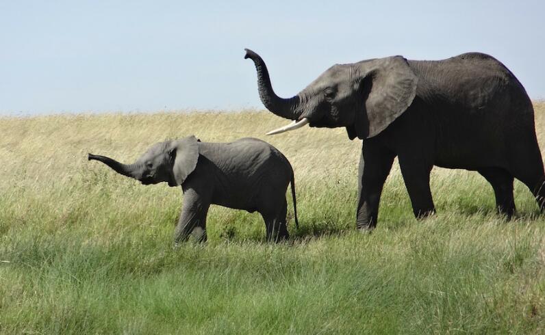
from keras.applications.vgg16 import VGG16
from keras.applications.vgg16 import preprocess_input

model = VGG16(weights='imagenet')
data_img = image.img_to_array(image.load_img('elephant.png'))
# VGG16预处理:RGB转BGR,并对每一个颜色通道去均值中心化
data_img = preprocess_input(data_img)
img_show = image.img_to_array(image.load_img('elephant.png'))

heatmaps(model, data_img, img_show)

elephant.png

结语

踩坑踩得我脚疼

以上这篇keras CNN卷积核可视化,热度图教程就是小编分享给大家的全部内容了，希望能给大家一个参考，也希望大家多多支持我们。