matplotlib中plt.hist()参数解释及应用实例

目录

• 一、plt.hist()参数详解
• 二、plt.hist()简单应用
• 三、plt.bar()综合应用
• 附官方参数解释

一、plt.hist()参数详解

简介：
plt.hist()：直方图，一种特殊的柱状图。
将统计值的范围分段，即将整个值的范围分成一系列间隔，然后计算每个间隔中有多少值。
直方图也可以被归一化以显示“相对”频率。 然后，它显示了属于几个类别中的每个类别的占比，其高度总和等于1。

import matplotlib as mpl
import matplotlib.pyplot as plt
from matplotlib.pyplot import MultipleLocator
from matplotlib import ticker
%matplotlib inline

plt.hist(x, bins=None, range=None, density=None, weights=None, cumulative=False, bottom=None, histtype='bar', align='mid', orientation='vertical', rwidth=None, log=False, color=None, label=None, stacked=False, normed=None, *, data=None, **kwargs)

常用参数解释：
x: 作直方图所要用的数据，必须是一维数组；多维数组可以先进行扁平化再作图；必选参数；
bins: 直方图的柱数，即要分的组数，默认为10；
range：元组(tuple)或None；剔除较大和较小的离群值，给出全局范围；如果为None，则默认为(x.min(), x.max())；即x轴的范围；
density：布尔值。如果为true，则返回的元组的第一个参数n将为频率而非默认的频数；
weights：与x形状相同的权重数组；将x中的每个元素乘以对应权重值再计数；如果normed或density取值为True，则会对权重进行归一化处理。这个参数可用于绘制已合并的数据的直方图；
cumulative：布尔值；如果为True，则计算累计频数；如果normed或density取值为True，则计算累计频率；
bottom：数组，标量值或None；每个柱子底部相对于y=0的位置。如果是标量值，则每个柱子相对于y=0向上/向下的偏移量相同。如果是数组，则根据数组元素取值移动对应的柱子；即直方图上下便宜距离；
histtype：{‘bar’, ‘barstacked’, ‘step’, ‘stepfilled’}；'bar’是传统的条形直方图；'barstacked’是堆叠的条形直方图；'step’是未填充的条形直方图，只有外边框；‘stepfilled’是有填充的直方图；当histtype取值为’step’或’stepfilled’，rwidth设置失效，即不能指定柱子之间的间隔，默认连接在一起；
align：{‘left’, ‘mid’, ‘right’}；‘left’：柱子的中心位于bins的左边缘；‘mid’：柱子位于bins左右边缘之间；‘right’：柱子的中心位于bins的右边缘；
orientation：{‘horizontal’, ‘vertical’}：如果取值为horizontal，则条形图将以y轴为基线，水平排列；简单理解为类似bar()转换成barh()，旋转90°；
rwidth：标量值或None。柱子的宽度占bins宽的比例；
log：布尔值。如果取值为True，则坐标轴的刻度为对数刻度；如果log为True且x是一维数组，则计数为0的取值将被剔除，仅返回非空的(frequency, bins, patches）；
color：具体颜色，数组（元素为颜色）或None。
label：字符串（序列）或None；有多个数据集时，用label参数做标注区分；
stacked：布尔值。如果取值为True，则输出的图为多个数据集堆叠累计的结果；如果取值为False且histtype=‘bar’或’step’，则多个数据集的柱子并排排列；
normed: 是否将得到的直方图向量归一化，即显示占比，默认为0，不归一化；不推荐使用，建议改用density参数；
edgecolor: 直方图边框颜色；
alpha: 透明度；

返回值（用参数接收返回值，便于设置数据标签）：
n：直方图向量，即每个分组下的统计值，是否归一化由参数normed设定。当normed取默认值时，n即为直方图各组内元素的数量（各组频数）；
bins: 返回各个bin的区间范围；
patches：返回每个bin里面包含的数据，是一个list。
其他参数与plt.bar()类似。

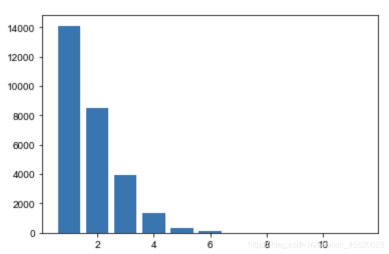
二、plt.hist()简单应用

import matplotlib.pyplot as plt
%matplotlib inline

# 最简单，只传递x，组数，宽度，范围
plt.hist(data13['carrier_no'], bins=11, rwidth=0.8, range=(1,12), align='left')
plt.show()

三、plt.bar()综合应用

import matplotlib as mpl
import matplotlib.pyplot as plt
from matplotlib.pyplot import MultipleLocator
from matplotlib import ticker
%matplotlib inline

plt.figure(figsize=(8,5), dpi=80)
# 拿参数接收hist返回值，主要用于记录分组返回的值，标记数据标签
n, bins, patches = plt.hist(data13['carrier_no'], bins=11, rwidth=0.8, range=(1,12), align='left', label='xx直方图')
for i in range(len(n)):
    plt.text(bins[i], n[i]*1.02, int(n[i]), fontsize=12, horizontalalignment="center") #打标签，在合适的位置标注每个直方图上面样本数
plt.ylim(0,16000)
plt.title('直方图')
plt.legend()
# plt.savefig('直方图'+'.png')
plt.show()

附官方参数解释

Parameters
----------
x : (n,) array or sequence of (n,) arrays
    Input values, this takes either a single array or a sequence of
    arrays which are not required to be of the same length.

bins : int or sequence or str, optional
    If an integer is given, ``bins + 1`` bin edges are calculated and
    returned, consistent with `numpy.histogram`.

    If `bins` is a sequence, gives bin edges, including left edge of
    first bin and right edge of last bin.  In this case, `bins` is
    returned unmodified.

    All but the last (righthand-most) bin is half-open.  In other
    words, if `bins` is::

        [1, 2, 3, 4]

    then the first bin is ``[1, 2)`` (including 1, but excluding 2) and
    the second ``[2, 3)``.  The last bin, however, is ``[3, 4]``, which
    *includes* 4.

    Unequally spaced bins are supported if *bins* is a sequence.

    With Numpy 1.11 or newer, you can alternatively provide a string
    describing a binning strategy, such as 'auto', 'sturges', 'fd',
    'doane', 'scott', 'rice' or 'sqrt', see
    `numpy.histogram`.

    The default is taken from :rc:`hist.bins`.

range : tuple or None, optional
    The lower and upper range of the bins. Lower and upper outliers
    are ignored. If not provided, *range* is ``(x.min(), x.max())``.
    Range has no effect if *bins* is a sequence.

    If *bins* is a sequence or *range* is specified, autoscaling
    is based on the specified bin range instead of the
    range of x.

    Default is ``None``

density : bool, optional
    If ``True``, the first element of the return tuple will
    be the counts normalized to form a probability density, i.e.,
    the area (or integral) under the histogram will sum to 1.
    This is achieved by dividing the count by the number of
    observations times the bin width and not dividing by the total
    number of observations. If *stacked* is also ``True``, the sum of
    the histograms is normalized to 1.

    Default is ``None`` for both *normed* and *density*. If either is
    set, then that value will be used. If neither are set, then the
    args will be treated as ``False``.

    If both *density* and *normed* are set an error is raised.

weights : (n, ) array_like or None, optional
    An array of weights, of the same shape as *x*.  Each value in *x*
    only contributes its associated weight towards the bin count
    (instead of 1).  If *normed* or *density* is ``True``,
    the weights are normalized, so that the integral of the density
    over the range remains 1.

    Default is ``None``.

    This parameter can be used to draw a histogram of data that has
    already been binned, e.g. using `np.histogram` (by treating each
    bin as a single point with a weight equal to its count) ::

        counts, bins = np.histogram(data)
        plt.hist(bins[:-1], bins, weights=counts)

    (or you may alternatively use `~.bar()`).

cumulative : bool, optional
    If ``True``, then a histogram is computed where each bin gives the
    counts in that bin plus all bins for smaller values. The last bin
    gives the total number of datapoints. If *normed* or *density*
    is also ``True`` then the histogram is normalized such that the
    last bin equals 1. If *cumulative* evaluates to less than 0
    (e.g., -1), the direction of accumulation is reversed.
    In this case, if *normed* and/or *density* is also ``True``, then
    the histogram is normalized such that the first bin equals 1.

    Default is ``False``

bottom : array_like, scalar, or None
    Location of the bottom baseline of each bin.  If a scalar,
    the base line for each bin is shifted by the same amount.
    If an array, each bin is shifted independently and the length
    of bottom must match the number of bins.  If None, defaults to 0.

    Default is ``None``

histtype : {'bar', 'barstacked', 'step',  'stepfilled'}, optional
    The type of histogram to draw.

    - 'bar' is a traditional bar-type histogram.  If multiple data
      are given the bars are arranged side by side.

    - 'barstacked' is a bar-type histogram where multiple
      data are stacked on top of each other.

    - 'step' generates a lineplot that is by default
      unfilled.

    - 'stepfilled' generates a lineplot that is by default
      filled.

    Default is 'bar'

align : {'left', 'mid', 'right'}, optional
    Controls how the histogram is plotted.

        - 'left': bars are centered on the left bin edges.

        - 'mid': bars are centered between the bin edges.

        - 'right': bars are centered on the right bin edges.

    Default is 'mid'

orientation : {'horizontal', 'vertical'}, optional
    If 'horizontal', `~matplotlib.pyplot.barh` will be used for
    bar-type histograms and the *bottom* kwarg will be the left edges.

rwidth : scalar or None, optional
    The relative width of the bars as a fraction of the bin width.  If
    ``None``, automatically compute the width.

    Ignored if *histtype* is 'step' or 'stepfilled'.

    Default is ``None``

log : bool, optional
    If ``True``, the histogram axis will be set to a log scale. If
    *log* is ``True`` and *x* is a 1D array, empty bins will be
    filtered out and only the non-empty ``(n, bins, patches)``
    will be returned.

    Default is ``False``

color : color or array_like of colors or None, optional
    Color spec or sequence of color specs, one per dataset.  Default
    (``None``) uses the standard line color sequence.

    Default is ``None``

label : str or None, optional
    String, or sequence of strings to match multiple datasets.  Bar
    charts yield multiple patches per dataset, but only the first gets
    the label, so that the legend command will work as expected.

    default is ``None``

stacked : bool, optional
    If ``True``, multiple data are stacked on top of each other If
    ``False`` multiple data are arranged side by side if histtype is
    'bar' or on top of each other if histtype is 'step'

    Default is ``False``

normed : bool, optional
    Deprecated; use the density keyword argument instead.

Returns
-------
n : array or list of arrays
    The values of the histogram bins. See *density* and *weights* for a
    description of the possible semantics.  If input *x* is an array,
    then this is an array of length *nbins*. If input is a sequence of
    arrays ``[data1, data2,..]``, then this is a list of arrays with
    the values of the histograms for each of the arrays in the same
    order.  The dtype of the array *n* (or of its element arrays) will
    always be float even if no weighting or normalization is used.

bins : array
    The edges of the bins. Length nbins + 1 (nbins left edges and right
    edge of last bin).  Always a single array even when multiple data
    sets are passed in.

patches : list or list of lists
    Silent list of individual patches used to create the histogram
    or list of such list if multiple input datasets.

Other Parameters
----------------
**kwargs : `~matplotlib.patches.Patch` properties

See also
--------
hist2d : 2D histograms

Notes
-----

.. note::
    In addition to the above described arguments, this function can take a
    **data** keyword argument. If such a **data** argument is given, the
    following arguments are replaced by **data[<arg>]**:

    * All arguments with the following names: 'weights', 'x'.

    Objects passed as **data** must support item access (``data[<arg>]``) and
    membership test (``<arg> in data``).

到此这篇关于matplotlib中plt.hist()参数解释及应用实例的文章就介绍到这了,更多相关matplotlib plt.hist()参数内容请搜索我们以前的文章或继续浏览下面的相关文章希望大家以后多多支持我们！