详解TensorFlow2实现线性回归

目录

• 概述
• MSE
• 线性回归
• 公式
• 梯度下降
• 线性回归实现
• 计算 MSE
• 梯度下降
• 迭代训练
• 主函数
• 完整代码

概述

线性回归 (Linear Regression) 是利用回归分析来确定两种或两种以上变量间相互依赖的定量关系.

对线性回归还不是很了解的同学可以看一下这篇文章:

python深度总结线性回归

MSE

均方误差 (Mean Square Error): 是用来描述连续误差的一种方法. 公式:

y_predict: 我们预测的值y_real: 真实值

线性回归

公式

w: weight, 权重系数

b: bias, 偏置顶

x: 特征值

y: 预测值

梯度下降

梯度下降 (Gradient Descent) 是一种优化算法. 参数会沿着梯度相反的方向前进, 以实现损失函数 (loss function) 的最小化.

计算公式:

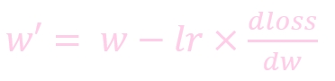
w: weight, 权重参数

w': 更新后的 weight

lr : learning rate, 学习率

dloss/dw: 损失函数对 w 求导

w: weight, 权重参数

w': 更新后的 weight

lr : learning rate, 学习率

dloss/dw: 损失函数对 b 求导

线性回归实现

计算 MSE

def calculate_MSE(w, b, points):
    """
    计算误差MSE
    :param w: weight, 权重
    :param b: bias, 偏置顶
    :param points: 数据
    :return: 返回MSE (Mean Square Error)
    """

    total_error = 0  # 存放总误差, 初始化为0

    # 遍历数据
    for i in range(len(points)):
        # 取出x, y
        x = points.iloc[i, 0]  # 第一列
        y = points.iloc[i, 1]  # 第二列

        # 计算MSE
        total_error += (y - (w * x + b)) ** 2  # 计总误差
        MSE = total_error / len(points)  # 计算平均误差

    # 返回MSE
    return MSE

梯度下降

def step_gradient(index, w_current, b_current, points, learning_rate=0.0001):
    """
    计算梯度下降, 跟新权重
    :param index: 现行迭代编号
    :param w_current: weight, 权重
    :param b_current: bias, 偏置顶
    :param points: 数据
    :param learning_rate: lr, 学习率 (默认值: 0.0001)
    :return: 返回跟新过后的参数数组
    """

    b_gradient = 0  # b的导, 初始化为0
    w_gradient = 0  # w的导, 初始化为0
    N = len(points)  # 数据长度

    # 遍历数据
    for i in range(len(points)):
        # 取出x, y
        x = points.iloc[i, 0]  # 第一列
        y = points.iloc[i, 1]  # 第二列

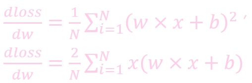
        # 计算w的导, w的导 = 2x(wx+b-y)
        w_gradient += (2 / N) * x * ((w_current * x + b_current) - y)

        # 计算b的导, b的导 = 2(wx+b-y)
        b_gradient += (2 / N) * ((w_current * x + b_current) - y)

    # 跟新w和b
    w_new = w_current - (learning_rate * w_gradient)  # 下降导数*学习率
    b_new = b_current - (learning_rate * b_gradient)  # 下降导数*学习率

    # 每迭代10次, 调试输出
    if index % 10 == 0:
        print("This is the {}th iterations w = {}, b = {}, error = {}"
              .format(index, w_new, b_new,
                      calculate_MSE(w_new, b_new, points)))

    # 返回更新后的权重和偏置顶
    return [w_new, b_new]

迭代训练

def runner(w_start, b_start, points, learning_rate, num_iterations):
    """
    迭代训练
    :param w_start: 初始weight
    :param b_start: 初始bias
    :param points: 数据
    :param learning_rate: 学习率
    :param num_iterations: 迭代次数
    :return: 训练好的权重和偏执顶
    """

    # 定义w_end, b_end, 存放返回权重
    w_end = w_start
    b_end = b_start

    # 更新权重
    for i in range(1, num_iterations + 1):
        w_end, b_end = step_gradient(i, w_end, b_end, points, learning_rate)

    # 返回训练好的b, w
    return [w_end, b_end]

主函数

def run():
    """
    主函数
    :return: 无返回值
    """

    # 读取数据
    data = pd.read_csv("data.csv")  

    # 定义超参数
    learning_rate = 0.00001  # 学习率
    w_initial = 0  # 权重初始化
    b_initial = 0  # 偏置顶初始化
    w_end = 0  # 存放返回结果
    b_end = 0  # 存放返回结果
    num_interations = 200  # 迭代次数

    # 调试输出初始误差
    print("Starting gradient descent at w = {}, b = {}, error = {}"
          .format(w_initial, b_initial, calculate_MSE(w_initial, b_initial, data)))
    print("Running...")

    # 得到训练好的值
    w_end, b_end = runner(w_initial, b_initial, data, learning_rate, num_interations, )

    # 调试输出训练后的误差
    print("\nAfter {} iterations w = {}, b = {}, error = {}"
          .format(num_interations, w_end, b_end, calculate_MSE(w_end, b_end, data)))

完整代码

import pandas as pd
import tensorflow as tf

def run():
    """
    主函数
    :return: 无返回值
    """

    # 读取数据
    data = pd.read_csv("data.csv")

    # 定义超参数
    learning_rate = 0.00001  # 学习率
    w_initial = 0  # 权重初始化
    b_initial = 0  # 偏置顶初始化
    w_end = 0  # 存放返回结果
    b_end = 0  # 存放返回结果
    num_interations = 200  # 迭代次数

    # 调试输出初始误差
    print("Starting gradient descent at w = {}, b = {}, error = {}"
          .format(w_initial, b_initial, calculate_MSE(w_initial, b_initial, data)))
    print("Running...")

    # 得到训练好的值
    w_end, b_end = runner(w_initial, b_initial, data, learning_rate, num_interations, )

    # 调试输出训练后的误差
    print("\nAfter {} iterations w = {}, b = {}, error = {}"
          .format(num_interations, w_end, b_end, calculate_MSE(w_end, b_end, data)))

def calculate_MSE(w, b, points):
    """
    计算误差MSE
    :param w: weight, 权重
    :param b: bias, 偏置顶
    :param points: 数据
    :return: 返回MSE (Mean Square Error)
    """

    total_error = 0  # 存放总误差, 初始化为0

    # 遍历数据
    for i in range(len(points)):
        # 取出x, y
        x = points.iloc[i, 0]  # 第一列
        y = points.iloc[i, 1]  # 第二列

        # 计算MSE
        total_error += (y - (w * x + b)) ** 2  # 计总误差
        MSE = total_error / len(points)  # 计算平均误差

    # 返回MSE
    return MSE

def step_gradient(index, w_current, b_current, points, learning_rate=0.0001):
    """
    计算梯度下降, 跟新权重
    :param index: 现行迭代编号
    :param w_current: weight, 权重
    :param b_current: bias, 偏置顶
    :param points: 数据
    :param learning_rate: lr, 学习率 (默认值: 0.0001)
    :return: 返回跟新过后的参数数组
    """

    b_gradient = 0  # b的导, 初始化为0
    w_gradient = 0  # w的导, 初始化为0
    N = len(points)  # 数据长度

    # 遍历数据
    for i in range(len(points)):
        # 取出x, y
        x = points.iloc[i, 0]  # 第一列
        y = points.iloc[i, 1]  # 第二列

        # 计算w的导, w的导 = 2x(wx+b-y)
        w_gradient += (2 / N) * x * ((w_current * x + b_current) - y)

        # 计算b的导, b的导 = 2(wx+b-y)
        b_gradient += (2 / N) * ((w_current * x + b_current) - y)

    # 跟新w和b
    w_new = w_current - (learning_rate * w_gradient)  # 下降导数*学习率
    b_new = b_current - (learning_rate * b_gradient)  # 下降导数*学习率

    # 每迭代10次, 调试输出
    if index % 10 == 0:
        print("This is the {}th iterations w = {}, b = {}, error = {}"
              .format(index, w_new, b_new,
                      calculate_MSE(w_new, b_new, points)))

    # 返回更新后的权重和偏置顶
    return [w_new, b_new]

def runner(w_start, b_start, points, learning_rate, num_iterations):
    """
    迭代训练
    :param w_start: 初始weight
    :param b_start: 初始bias
    :param points: 数据
    :param learning_rate: 学习率
    :param num_iterations: 迭代次数
    :return: 训练好的权重和偏执顶
    """

    # 定义w_end, b_end, 存放返回权重
    w_end = w_start
    b_end = b_start

    # 更新权重
    for i in range(1, num_iterations + 1):
        w_end, b_end = step_gradient(i, w_end, b_end, points, learning_rate)

    # 返回训练好的b, w
    return [w_end, b_end]

if __name__ == "__main__":  # 判断是否为直接运行
    # 执行主函数
    run()

输出结果:

Starting gradient descent at w = 0, b = 0, error = 5611.166153823905
Running...
This is the 10th iterations w = 0.5954939346814911, b = 0.011748797759247776, error = 2077.4540105037636
This is the 20th iterations w = 0.9515563561471605, b = 0.018802975867006404, error = 814.0851271130122
This is the 30th iterations w = 1.1644557718428263, b = 0.023050105300353223, error = 362.4068500146176
This is the 40th iterations w = 1.291753898278705, b = 0.02561881917471017, error = 200.92329896151622
This is the 50th iterations w = 1.3678685455519075, b = 0.027183959773995233, error = 143.18984477036037
This is the 60th iterations w = 1.4133791147591803, b = 0.02814903475888354, error = 122.54901023376003
This is the 70th iterations w = 1.4405906232245687, b = 0.028755312994862656, error = 115.16948797045545
This is the 80th iterations w = 1.4568605956220553, b = 0.029147056093611835, error = 112.53113537539161
This is the 90th iterations w = 1.4665883081088924, b = 0.029410522232548166, error = 111.58784050644537
This is the 100th iterations w = 1.4724042147529013, b = 0.029597287663210802, error = 111.25056079777497
This is the 110th iterations w = 1.475881139890538, b = 0.029738191313600983, error = 111.12994295811941
This is the 120th iterations w = 1.477959520545057, b = 0.02985167266801462, error = 111.08678583026905
This is the 130th iterations w = 1.479201671130221, b = 0.029948757225817496, error = 111.07132237076124
This is the 140th iterations w = 1.4799438156483897, b = 0.03003603745100295, error = 111.06575992136905
This is the 150th iterations w = 1.480386992125614, b = 0.030117455167888288, error = 111.06373727064113
This is the 160th iterations w = 1.4806514069946144, b = 0.030195367306897165, error = 111.0629801653088
This is the 170th iterations w = 1.4808089351476725, b = 0.030271183144693698, error = 111.06267551686379
This is the 180th iterations w = 1.4809025526554018, b = 0.030345745328433527, error = 111.0625326308038
This is the 190th iterations w = 1.4809579561496398, b = 0.030419557701150367, error = 111.0624475783524
This is the 200th iterations w = 1.480990510387525, b = 0.030492921525124016, error = 111.06238320300855
This is the 210th iterations w = 1.4810094024003952, b = 0.030566016933760057, error = 111.06232622062124
This is the 220th iterations w = 1.4810201253791957, b = 0.030638951634017437, error = 111.0622718818556
This is the 230th iterations w = 1.4810259638611891, b = 0.030711790026994222, error = 111.06221848873447
This is the 240th iterations w = 1.481028881765914, b = 0.030784570619965538, error = 111.06216543419914
This is the 250th iterations w = 1.4810300533774932, b = 0.030857316437543122, error = 111.06211250121454
This is the 260th iterations w = 1.4810301808342632, b = 0.03093004124680784, error = 111.06205961218657
This is the 270th iterations w = 1.4810296839649824, b = 0.031002753279495907, error = 111.06200673937376
This is the 280th iterations w = 1.4810288137973704, b = 0.031075457457601333, error = 111.06195387285815
This is the 290th iterations w = 1.48102772042814, b = 0.031148156724127858, error = 111.06190100909376
This is the 300th iterations w = 1.4810264936044433, b = 0.03122085283878386, error = 111.06184814681296
This is the 310th iterations w = 1.4810251869886903, b = 0.0312935468537513, error = 111.06179528556238
This is the 320th iterations w = 1.4810238326671836, b = 0.031366239398161695, error = 111.0617424251801
This is the 330th iterations w = 1.4810224498252484, b = 0.031438930848192506, error = 111.06168956560795
This is the 340th iterations w = 1.481021049934344, b = 0.03151162142877266, error = 111.06163670682551
This is the 350th iterations w = 1.4810196398535866, b = 0.03158431127439525, error = 111.06158384882504
This is the 360th iterations w = 1.4810182236842395, b = 0.03165700046547913, error = 111.0615309916041
This is the 370th iterations w = 1.4810168038785667, b = 0.031729689050110664, error = 111.06147813516172
This is the 380th iterations w = 1.4810153819028469, b = 0.03180237705704362, error = 111.06142527949757
This is the 390th iterations w = 1.48101395863381, b = 0.03187506450347233, error = 111.06137242461139
This is the 400th iterations w = 1.48101253459568, b = 0.03194775139967933, error = 111.06131957050317
This is the 410th iterations w = 1.4810111101019028, b = 0.03202043775181446, error = 111.06126671717288
This is the 420th iterations w = 1.4810096853398989, b = 0.032093123563556446, error = 111.06121386462064
This is the 430th iterations w = 1.4810082604217312, b = 0.032165808837106485, error = 111.06116101284626
This is the 440th iterations w = 1.481006835414406, b = 0.03223849357378233, error = 111.06110816184975
This is the 450th iterations w = 1.4810054103579875, b = 0.03231117777437349, error = 111.06105531163115
This is the 460th iterations w = 1.4810039852764323, b = 0.0323838614393536, error = 111.06100246219052
This is the 470th iterations w = 1.4810025601840635, b = 0.032456544569007456, error = 111.0609496135277
This is the 480th iterations w = 1.4810011350894463, b = 0.03252922716350693, error = 111.06089676564281
This is the 490th iterations w = 1.4809997099977015, b = 0.032601909222956374, error = 111.06084391853577
This is the 500th iterations w = 1.4809982849118903, b = 0.032674590747419754, error = 111.0607910722065

After 500 iterations w = 1.4809982849118903, b = 0.032674590747419754, error = 111.0607910722065

到此这篇关于详解TensorFlow2实现线性回归的文章就介绍到这了,更多相关TensorFlow2线性回归内容请搜索我们以前的文章或继续浏览下面的相关文章希望大家以后多多支持我们！