python实现低通滤波器代码

低通滤波器实验代码，这是参考别人网上的代码，所以自己也分享一下，共同进步

# -*- coding: utf-8 -*-

import numpy as np
from scipy.signal import butter, lfilter, freqz
import matplotlib.pyplot as plt

def butter_lowpass(cutoff, fs, order=5):
 nyq = 0.5 * fs
 normal_cutoff = cutoff / nyq
 b, a = butter(order, normal_cutoff, btype='low', analog=False)
 return b, a

def butter_lowpass_filter(data, cutoff, fs, order=5):
 b, a = butter_lowpass(cutoff, fs, order=order)
 y = lfilter(b, a, data)
 return y # Filter requirements.

order = 6
fs = 30.0 # sample rate, Hz
cutoff = 3.667 # desired cutoff frequency of the filter, Hz # Get the filter coefficients so we can check its frequency response.
b, a = butter_lowpass(cutoff, fs, order) # Plot the frequency response.
w, h = freqz(b, a, worN=800)
plt.subplot(2, 1, 1)
plt.plot(0.5*fs*w/np.pi, np.abs(h), 'b')
plt.plot(cutoff, 0.5*np.sqrt(2), 'ko')
plt.axvline(cutoff, color='k')
plt.xlim(0, 0.5*fs)
plt.title("Lowpass Filter Frequency Response")
plt.xlabel('Frequency [Hz]')
plt.grid() # Demonstrate the use of the filter. # First make some data to be filtered.
T = 5.0 # seconds
n = int(T * fs) # total number of samples
t = np.linspace(0, T, n, endpoint=False) # "Noisy" data. We want to recover the 1.2 Hz signal from this.
data = np.sin(1.2*2*np.pi*t) + 1.5*np.cos(9*2*np.pi*t) + 0.5*np.sin(12.0*2*np.pi*t) # Filter the data, and plot both the original and filtered signals.
y = butter_lowpass_filter(data, cutoff, fs, order)
plt.subplot(2, 1, 2)
plt.plot(t, data, 'b-', label='data')
plt.plot(t, y, 'g-', linewidth=2, label='filtered data')
plt.xlabel('Time [sec]')
plt.grid()
plt.legend()
plt.subplots_adjust(hspace=0.35)
plt.show()

实际代码，没有整理，可以读取txt文本文件，然后进行低通滤波，并将滤波前后的波形和FFT变换都显示出来

# -*- coding: utf-8 -*-

import numpy as np
from scipy.signal import butter, lfilter, freqz
import matplotlib.pyplot as plt
import os

def butter_lowpass(cutoff, fs, order=5):
 nyq = 0.5 * fs
 normal_cutoff = cutoff / nyq
 b, a = butter(order, normal_cutoff, btype='low', analog=False)
 return b, a

def butter_lowpass_filter(data, cutoff, fs, order=5):
 b, a = butter_lowpass(cutoff, fs, order=order)
 y = lfilter(b, a, data)
 return y # Filter requirements.

order = 5
fs = 100000.0 # sample rate, Hz
cutoff = 1000 # desired cutoff frequency of the filter, Hz # Get the filter coefficients so we can check its frequency response.
# b, a = butter_lowpass(cutoff, fs, order) # Plot the frequency response.
# w, h = freqz(b, a, worN=1000)
# plt.subplot(3, 1, 1)
# plt.plot(0.5*fs*w/np.pi, np.abs(h), 'b')
# plt.plot(cutoff, 0.5*np.sqrt(2), 'ko')
# plt.axvline(cutoff, color='k')
# plt.xlim(0, 1000)
# plt.title("Lowpass Filter Frequency Response")
# plt.xlabel('Frequency [Hz]')
# plt.grid() # Demonstrate the use of the filter. # First make some data to be filtered.
# T = 5.0 # seconds
# n = int(T * fs) # total number of samples
# t = np.linspace(0, T, n, endpoint=False) # "Noisy" data. We want to recover the 1.2 Hz signal from this.
# # data = np.sin(1.2*2*np.pi*t) + 1.5*np.cos(9*2*np.pi*t) + 0.5*np.sin(12.0*2*np.pi*t) # Filter the data, and plot both the original and filtered signals.

path = "*****"

for file in os.listdir(path):
 if file.endswith("txt"):
  data=[]
  filePath = os.path.join(path, file)
  with open(filePath, 'r') as f:
   lines = f.readlines()[8:]
   for line in lines:
    # print(line)
    data.append(float(line)*100)
  # print(len(data))
  t1=[i*10 for i in range(len(data))]
  plt.subplot(231)
  # plt.plot(range(len(data)), data)
  plt.plot(t1, data, linewidth=2,label='original data')
  # plt.title('ori wave', fontsize=10, color='#F08080')
  plt.xlabel('Time [us]')
  plt.legend()

  # filter_data = data[30000:35000]
  # filter_data=data[60000:80000]
  # filter_data2=data[60000:80000]
  # filter_data = data[80000:100000]
  # filter_data = data[100000:120000]
  filter_data = data[120000:140000]

  filter_data2=filter_data
  t2=[i*10 for i in range(len(filter_data))]
  plt.subplot(232)
  plt.plot(t2, filter_data, linewidth=2,label='cut off wave before filter')
  plt.xlabel('Time [us]')
  plt.legend()
  # plt.title('cut off wave', fontsize=10, color='#F08080')

  # filter_data=zip(range(1,len(data),int(fs/len(data))),data)
  # print(filter_data)
  n1 = len(filter_data)
  Yamp1 = abs(np.fft.fft(filter_data) / (n1 / 2))
  Yamp1 = Yamp1[range(len(Yamp1) // 2)]
  # x_axis=range(0,n//2,int(fs/len
  # 计算最大赋值点频率
  max1 = np.max(Yamp1)
  max1_index = np.where(Yamp1 == max1)
  if (len(max1_index[0]) == 2):
   print((max1_index[0][0] )* fs / n1, (max1_index[0][1]) * fs / n1)
  else:
   Y_second = Yamp1
   Y_second = np.sort(Y_second)
   print(np.where(Yamp1 == max1)[0] * fs / n1,
     (np.where(Yamp1 == Y_second[-2])[0]) * fs / n1)
  N1 = len(Yamp1)
  # print(N1)
  x_axis1 = [i * fs / n1 for i in range(N1)]

  plt.subplot(233)
  plt.plot(x_axis1[:300], Yamp1[:300], linewidth=2,label='FFT data')
  plt.xlabel('Frequence [Hz]')
  # plt.title('FFT', fontsize=10, color='#F08080')
  plt.legend()
  # plt.savefig(filePath.replace("txt", "png"))
  # plt.close()
  # plt.show()

  Y = butter_lowpass_filter(filter_data2, cutoff, fs, order)
  n3 = len(Y)
  t3 = [i * 10 for i in range(n3)]
  plt.subplot(235)
  plt.plot(t3, Y, linewidth=2, label='cut off wave after filter')
  plt.xlabel('Time [us]')
  plt.legend()
  Yamp2 = abs(np.fft.fft(Y) / (n3 / 2))
  Yamp2 = Yamp2[range(len(Yamp2) // 2)]
  # x_axis = range(0, n // 2, int(fs / len(Yamp)))
  max2 = np.max(Yamp2)
  max2_index = np.where(Yamp2 == max2)
  if (len(max2_index[0]) == 2):
   print(max2, max2_index[0][0] * fs / n3, max2_index[0][1] * fs / n3)
  else:
   Y_second2 = Yamp2
   Y_second2 = np.sort(Y_second2)
   print((np.where(Yamp2 == max2)[0]) * fs / n3,
     (np.where(Yamp2 == Y_second2[-2])[0]) * fs / n3)
  N2=len(Yamp2)
  # print(N2)
  x_axis2 = [i * fs / n3 for i in range(N2)]

  plt.subplot(236)
  plt.plot(x_axis2[:300], Yamp2[:300],linewidth=2, label='FFT data after filter')
  plt.xlabel('Frequence [Hz]')
  # plt.title('FFT after low_filter', fontsize=10, color='#F08080')
  plt.legend()
  # plt.show()
  plt.savefig(filePath.replace("txt", "png"))
  plt.close()
  print('*'*50)

  # plt.subplot(3, 1, 2)
  # plt.plot(range(len(data)), data, 'b-', linewidth=2,label='original data')
  # plt.grid()
  # plt.legend()
  #
  # plt.subplot(3, 1, 3)
  # plt.plot(range(len(y)), y, 'g-', linewidth=2, label='filtered data')
  # plt.xlabel('Time')
  # plt.grid()
  # plt.legend()
  # plt.subplots_adjust(hspace=0.35)
  # plt.show()
  '''
  # Y_fft = Y[60000:80000]
  Y_fft = Y
  # Y_fft = Y[80000:100000]
  # Y_fft = Y[100000:120000]
  # Y_fft = Y[120000:140000]
  n = len(Y_fft)
  Yamp = np.fft.fft(Y_fft)/(n/2)
  Yamp = Yamp[range(len(Yamp)//2)]

  max = np.max(Yamp)
  # print(max, np.where(Yamp == max))

  Y_second = Yamp
  Y_second=np.sort(Y_second)
  print(float(np.where(Yamp == max)[0])* fs / len(Yamp),float(np.where(Yamp==Y_second[-2])[0])* fs / len(Yamp))
  # print(float(np.where(Yamp == max)[0]) * fs / len(Yamp))
  '''

补充拓展：浅谈opencv的理想低通滤波器和巴特沃斯低通滤波器

低通滤波器

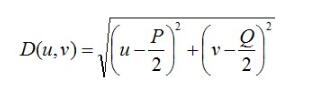
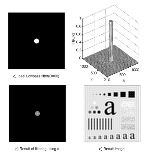
1.理想的低通滤波器

其中，D0表示通带的半径。D(u,v)的计算方式也就是两点间的距离，很简单就能得到。

使用低通滤波器所得到的结果如下所示。低通滤波器滤除了高频成分，所以使得图像模糊。由于理想低通滤波器的过度特性过于急峻，所以会产生了振铃现象。

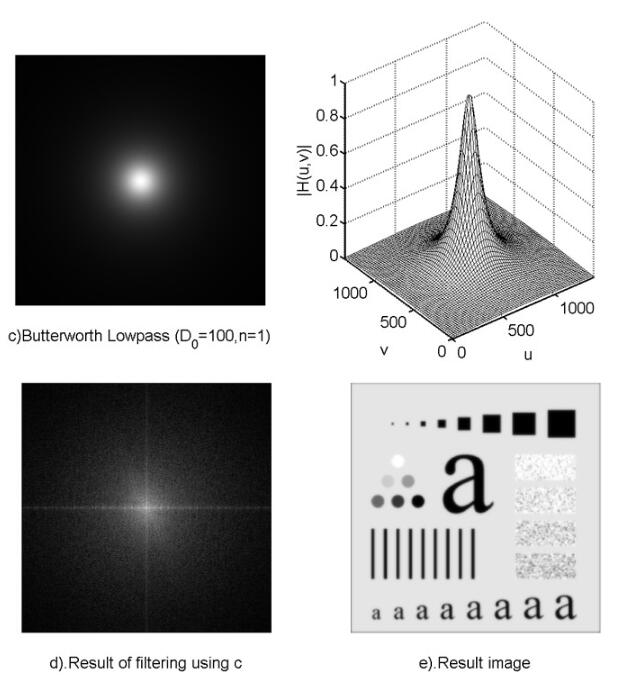
2.巴特沃斯低通滤波器

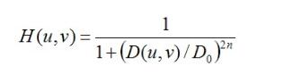
同样的，D0表示通带的半径，n表示的是巴特沃斯滤波器的次数。随着次数的增加，振铃现象会越来越明显。

void ideal_Low_Pass_Filter(Mat src){
	Mat img;
	cvtColor(src, img, CV_BGR2GRAY);
	imshow("img",img);
	//调整图像加速傅里叶变换
	int M = getOptimalDFTSize(img.rows);
	int N = getOptimalDFTSize(img.cols);
	Mat padded;
	copyMakeBorder(img, padded, 0, M - img.rows, 0, N - img.cols, BORDER_CONSTANT, Scalar::all(0));
	//记录傅里叶变换的实部和虚部
	Mat planes[] = { Mat_<float>(padded), Mat::zeros(padded.size(), CV_32F) };
	Mat complexImg;
	merge(planes, 2, complexImg);
	//进行傅里叶变换
	dft(complexImg, complexImg);
	//获取图像
	Mat mag = complexImg;
	mag = mag(Rect(0, 0, mag.cols & -2, mag.rows & -2));//这里为什么&上-2具体查看opencv文档
	//其实是为了把行和列变成偶数 -2的二进制是11111111.......10 最后一位是0
	//获取中心点坐标
	int cx = mag.cols / 2;
	int cy = mag.rows / 2;
	//调整频域
	Mat tmp;
	Mat q0(mag, Rect(0, 0, cx, cy));
	Mat q1(mag, Rect(cx, 0, cx, cy));
	Mat q2(mag, Rect(0, cy, cx, cy));
	Mat q3(mag, Rect(cx, cy, cx, cy));

	q0.copyTo(tmp);
	q3.copyTo(q0);
	tmp.copyTo(q3);

	q1.copyTo(tmp);
	q2.copyTo(q1);
	tmp.copyTo(q2);
	//Do为自己设定的阀值具体看公式
	double D0 = 60;
	//处理按公式保留中心部分
	for (int y = 0; y < mag.rows; y++){
		double* data = mag.ptr<double>(y);
		for (int x = 0; x < mag.cols; x++){
			double d = sqrt(pow((y - cy),2) + pow((x - cx),2));
			if (d <= D0){

			}
			else{
				data[x] = 0;
			}
		}
	}
	//再调整频域
	q0.copyTo(tmp);
	q3.copyTo(q0);
	tmp.copyTo(q3);
	q1.copyTo(tmp);
	q2.copyTo(q1);
	tmp.copyTo(q2);
	//逆变换
	Mat invDFT, invDFTcvt;
	idft(mag, invDFT, DFT_SCALE | DFT_REAL_OUTPUT); // Applying IDFT
	invDFT.convertTo(invDFTcvt, CV_8U);
	imshow("理想低通滤波器", invDFTcvt);
}

void Butterworth_Low_Paass_Filter(Mat src){
	int n = 1;//表示巴特沃斯滤波器的次数
	//H = 1 / (1+(D/D0)^2n)
	Mat img;
	cvtColor(src, img, CV_BGR2GRAY);
	imshow("img", img);
	//调整图像加速傅里叶变换
	int M = getOptimalDFTSize(img.rows);
	int N = getOptimalDFTSize(img.cols);
	Mat padded;
	copyMakeBorder(img, padded, 0, M - img.rows, 0, N - img.cols, BORDER_CONSTANT, Scalar::all(0));

	Mat planes[] = { Mat_<float>(padded), Mat::zeros(padded.size(), CV_32F) };
	Mat complexImg;
	merge(planes, 2, complexImg);

	dft(complexImg, complexImg);

	Mat mag = complexImg;
	mag = mag(Rect(0, 0, mag.cols & -2, mag.rows & -2));

	int cx = mag.cols / 2;
	int cy = mag.rows / 2;

	Mat tmp;
	Mat q0(mag, Rect(0, 0, cx, cy));
	Mat q1(mag, Rect(cx, 0, cx, cy));
	Mat q2(mag, Rect(0, cy, cx, cy));
	Mat q3(mag, Rect(cx, cy, cx, cy));

	q0.copyTo(tmp);
	q3.copyTo(q0);
	tmp.copyTo(q3);

	q1.copyTo(tmp);
	q2.copyTo(q1);
	tmp.copyTo(q2);

	double D0 = 100;

	for (int y = 0; y < mag.rows; y++){
		double* data = mag.ptr<double>(y);
		for (int x = 0; x < mag.cols; x++){
			//cout << data[x] << endl;
			double d = sqrt(pow((y - cy), 2) + pow((x - cx), 2));
			//cout << d << endl;
			double h = 1.0 / (1 + pow(d / D0, 2 * n));
			if (h <= 0.5){
				data[x] = 0;
			}
			else{
				//data[x] = data[x]*0.5;
				//cout << h << endl;
			}

			//cout << data[x] << endl;
		}
	}
	q0.copyTo(tmp);
	q3.copyTo(q0);
	tmp.copyTo(q3);
	q1.copyTo(tmp);
	q2.copyTo(q1);
	tmp.copyTo(q2);
	//逆变换
	Mat invDFT, invDFTcvt;
	idft(complexImg, invDFT, DFT_SCALE | DFT_REAL_OUTPUT); // Applying IDFT
	invDFT.convertTo(invDFTcvt, CV_8U);
	imshow("巴特沃斯低通滤波器", invDFTcvt);
}

以上这篇python实现低通滤波器代码就是小编分享给大家的全部内容了，希望能给大家一个参考，也希望大家多多支持我们。